7th Grade- Creating a Shopping Budget List in Microsoft Excel

 Major Topic: Microsoft Excel

Class/Classes: 1-2 class periods

NETS for students

3.  Research and Information Fluency

• Students apply digital tools to gather, evaluate, and use information. \

4. Critical Thinking, Problem Solving, and Decision Making

•  Students use critical thinking skills to plan and conduct research, manage projects, solve problems, and make informed decisions using appropriate digital tools and resources

Materials:

• Microsoft Excel
• Microsoft Excel Notes (PowerPoint)- Student and Teacher Versions
• Excel Shopping Budget Tutorial
• Projector
• Electronic Whiteboard 
• Excel Shopping Budget Grade Sheet

Motivation:

• Have Microsoft Excel Open as well as the Microsoft Excel Notes (PowerPoint)-Student and Teacher Versions. Go over the notes PowerPoint while students fill in the blanks.

Activity:

• Make one copy per student of the Microsoft Excel Notes for Students. Have the Teacher’s version open in the front of the room. Go over the notes and demonstrate as you discuss each slide.

• Hand out the Excel Shopping Budget Tutorial (PDF Download). Have students follow the directions. (tutorial shown below).

• Tips: Before they start this tutorial show your students the various components of Microsoft Excel. Demonstrate: rows, columns, cell reference, formulas, text formatting, etc. to make them more comfortable using this program. This tutorial is just a basic intro as to what Microsoft Excel can do.

Tutorial:

Shopping Budget- Microsoft Excel

7^th grade

Directions: Follow the below steps to create a Shopping Budget Worksheet in Microsoft Excel.


Open Microsoft Excel from your desktop and save this new workbook as "MyBudget" in your student folder.

1. In Cell A1 type: Shopping Budget.

2. Merge and Center by selecting cells A1- F1 and select the Merge and Center Button located on the Home Tab (Microsoft 2007 & 2010).

Merge and center by selecting cells

3. Use the fill bucket and select a fill color to change the heading color (The cells you just merged in step 2). Change the color and style of the font (Size of font no smaller than 18 and no larger than 40).

Change font style, size and color under Home Tab

4. In cell

A3 type My Budget:

A4 type Total Cost:

A5 type Difference Total:

5. In cells
A7 type PERSON TO SHOP FOR
B7 type BUDGETED AMOUNT
C7 type AMOUNT SPENT
D7 type DIFFERENCE


Bold the text and make all uppercase. Now is a good time to save!


6. Starting in cell A9 (staying in column A) list 5-10 people you would like to shop for (this could be a list for birthdays, Christmas, etc.) and how much you wan to spend on each person. You do not need to add dollar signs! Please wait until step 8 for directions!
Example:

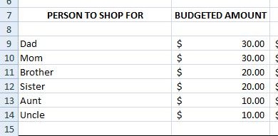Example of family and friends you can list. Please feel free to add "real" names

7.  Now, fictitiously make up amounts that you actually spent (you can spend more or less on each person)

Example:

!!! DO NOT ADD ANY NUMBERS IN THE DIFFERENCE COLUMN!!!

8. To convert numbers into dollar amounts, highlight all the cells that contain a number and click on the $ button on the Home Tab under Number Formatting:

Don't manually type in dollar signs- quickly add them in with the $ button on the home tab

9. Now is time to add calculations! In cell D (under the "DIFFERENCE" column), use the following equation, making sure that you start with the = sign first! =B9-C9

Copy and paste the equation to the remainder of the cells. Copy (or ctrl C) highlight the cells you need a formula in under the Difference Column. Paste (Ctrl V) the formula into the selected cells.

10. Now it's time to tally up the totals! Select cell B3 and click the "Insert Function" (looks like fx) button to begin the formula:

A dialog box then opens. Select the SUM function. Now is a good time to save!

The Sum function is usually under the "most recently used" category

Notice how the formula bar automatically adds "=sum"? 

11. A new dialog box "Function Arguments" opens up. This is where you will select your cells that you want to add together. 

 

12. Click the box to the right of the "Number 1" input box:

The box then collapses and you are free to select the cells that you want to add to this formula.

13. Highlight all the cells that have a currency amount under Budgeted Amount.

For example, the sum of cells B9-B14 would be the Budget amount I was looking for:

14. Open the "Function Arguments" dialog box up by pressing the same "Range of Cells Button" to expand the dialog box and click OK. The number in cell B3 should be the sum of all the cells that you have budgeted money for.

Now is a good time to save!

Put your practice to work!

15. Repeat steps 10-14 to find out the totals for Total Cost (cell B4) and Difference Total (cell B5)!

***Note: Make sure you find the SUM of the corresponding cells to Total Cost and Difference Total****

Add dollar signs to all that is needed!

16. Insert a clip art image to represent what your shopping budget is for. (Insert Tab --> Clip Art) Do not place your image over text, and keep the clip art relative!

17. Add a border around your table by selecting all the cells in your Budget Spreadsheet and click on the Borders Button on the Home Tab (Look for Thick Box Borders):

18. Change some other features such as text and cell fill (make at least 2 changes on your own.) 

19. Change the orientation of the page. Go to Page Layout --> Orientation --> Landscape:

20. Print Preview. If needed make appropriate adjustments to make the Shopping Budget print on one page. See image below:

Select Page Setup and then Fit to 1 page if needed.

21. Print once you have permission.